CSCI 2824 Lecture 21: Growth of Functions

Studying the growth of functions is an important part of the analysis of algorithms.

Take a look at the two codes below:

Linear Loop

for (i=0; i < n; ++i){
 sleep(1); /*-- Sleep for one second --*/
}

For n=10 , the program takes roughly 10s to run. Contrast the program above with this one:

Quadratic Loop

for (i=0; i < n; ++i){
  for (j=0; j < n; ++j){
    sleep(0.01); /*-- sleep 10 milli seconds --*/
  }
}

For n=10 , the program above takes 10 *.01 = .1s to run. Comparing the expected running times of the programs:

n	Linear	Quadratic	Comparison
10	10	.1	100x speedup
100	100	100	same
1000	1000	10,000	10x slowdown
10000	10000		100x slowdown

As increases, the quadratic loop gets slower and slower than the linear loop.

Let us increase the delay in each linear loop iteration to 10s and decrease the delay in quadratic loop to milli seconds (0.001 s). How does the table above change??

Answer

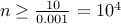The linear loop's running time for given input is roughly 10n seconds and the quadratic loop is 0.001 n^2 . But for $n geq frac{10}{0.001} = 10^4$ , the linear loop will once again be faster than the quadratic and remain so for larger values of .

Running Time Complexity of Algorithms

There are two basic rules we follow when comparing running times or analyzing running times of algorithms.

We only care about trends as input size tends to . In other words, the performance of algorithms often varies unpredictably for small input sizes. So we only care about the time complexity as they grow larger.

We do not care about constant factors: Algorithm implementation on x86 machine with 2 GHz clock frequency and 8 GB RAM may be much slower than a machine with 1 GHz clock and 4 GB RAM. But this slowdown often is a constant factor. It will roughly be some factor say times faster on the faster processor. But we do not care about these constant factors.

In terms of trends, we say that the linear loop in the example above has a running time complexity of O(n) (pronounced Big-OH of or Order ). And quadratic loop above has a complexity of O(n^2) .

Informally, O(n) can refer to running times that could in reality be any number of functions including:

or
$f_3(n) = 1000 n + 2 sqrt{n} sin(2 pi n)$ .
.

All we care about in these functions is that: as grows larger and larger, beyond n > N_0 for some large number N_0 , the dominant term in the function is with a constant factor in front of it. The remaining terms matter less and less as increases, and eventually stop being the dominant terms.

Let us now define the Big-OH notation.

Big-OH Notation

Given a function f: N rightarrow N , and g: N rightarrow N we write f in O(g) iff there exists a number N_0 such that for all n > N_0 ,

f(n) leq K g(n), mbox{for some constant} K

Note that O(g(n)) denotes a set of functions which satisfy the definition above.

In other words, we have that asymptotically as n rightarrow infty , g(n) grows at least as fast as f(n) (if not faster) as .

Eg., we have f(n) = 0.1 n being in the set O(n^2) . Beyond n geq 10 , we see that f(n) = 0.1 n leq n^2 .

Questions for class

Is ?
Is ?
$f_3(n): 2.5 n^{2.5} + 10 n^{1.5} - 132 in O(n^2)$ ?
what are all the functions in ?

Let us now answer these questions.

Answers

Yes. We have for , we have . Therefore, .
Yes. Once again, for , we have . Therefore, .
No. No matter, how high we set the constant , we $n^{2.5}$ , the dominant term of cannot be domainted by .
A function if eventually for some , . Therefore, any function that is eventually upper bounded by a constant will be in . Examples include: , , $h(n): frac{1}{n+1}$ , and so on.

Example # 2.

Is $2^{1.5n} in O(2^n)$ ?

Answer

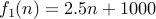
This is an interesting question. Can we find a constant such that $2^{1.5n} leq K 2^n$ for all n geq N_0 ? To understand, let us call m = 2.5^n . We have $2.5^{1.5n} = m^{1.5}$ . We are asking the question if $m in O(m^{1.5})$ ? The answer is no.

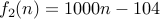
Is 100 * 2^n in O(2^n) ?

Answer

Once again, let us call 2^n as . We are asking now if 100m in O(m) , and the answer is yes.

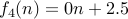
Is $2^{n} in O(2^{2n})$ ?

Answer

Again, let us call m = 2^n . We have $2^{2n} = m^2$ . We are asking if m in O(m^2) . The answer is yes.

Big-Omega and Big-Theta

Just like Big-Oh, we can define Big-Omega Omega(..) to denote lower bounds.

Big-Omega

We say that f(n) in Omega(g(n)) if and only if there is a N > 0 and a constant K > 0 such that

f(n) geq K g(n)

In other words, informally we say that the function is lower bounded asymptotically by (upto a constant factor).

Exampls

1. n in Omega(n)

We can choose N = 1 and K = 1 . We conclude (trivially) that n geq n for all n geq 1 .

2. n in Omega(sqrt{n}) .

We can choose N = 2 and K = 1 , we conclude that n geq sqrt{n} for all n geq 2 .

3. What are all the functions in Omega(n) , give a succinct description?

Any function whose growth is super-linear. Examples include $n^2, n^{1.2}, 5n + 10, nlog(n), ldots$ .

4. Is the following function in O(n^2) ? Is it in Omega(n^2) ?

$f(n) = left{ begin{array}{l} n^2, n mbox{is odd} sin^2 n, n mbox{even} end{array} right.$

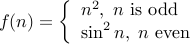
Since we are concerned about the asymptotics of the function: for the upper bound we should focus on f(n) = n^2 when is odd. Therefore, f(n) in O(n^2) . But for lower bound, we should look at f(n) = sin^2 n when is even. Therefore f notin Omega(n^2) .

We say that f(n) in Theta(g(n)) if f(n) in O(g(n)) cap Omega(g(n)) .

Note

It is common to write f(n) = O(g(n)) or f(n) = Theta (g(n)) often instead of f(n) in O(g(n)) . But the latter is more sound since O(g(n)) strictly speaking is not a function but a set of functions that are all upper bounded by g(n) .