A fundamental way to describe an object is to specify its topology: how many pieces or holes it contains, whether or not it is connected, etc. In the real world, this might appear to be a lost cause, as data are both limited in extent and quantized in space and time, and topology is fundamentally an infinite-precision notion.
There are, however, a variety of ways to glean useful information about the topological properties of a manifold from a finite number of finite-precision points upon it. For example, one can analyze the properties of the point-set data - e.g., the number of components and holes, and their sizes - at a variety of different precisions, and then deduce the topology from the limiting behavior of those curves. One can exploit connectedness, continuity, and lacunarity to separate signals from different dynamical regimes, and one can compute the Conley index of a dataset in order to find and formally verify the existence of periodic orbits. The remainder of this document explains and demonstrates some of these ideas.
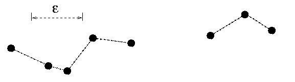
An epsilon chain is a finite sequence of points x_0 ... x_N that are separated by distances of epsilon or less: that is, |x_i - x_i+1| < epsilon. Two points are epsilon connected if there is an epsilon chain joining them. Any two points in an epsilon-connected set can be linked by an epsilon chain. The set shown in the image below, for instance, contains eight points:
|
For the purposes of this work, we define several fundamental quantities: the number C(epsilon) and maximum diameter D(epsilon) of the epsilon-connected components in a set, as well as the number I(epsilon) of epsilon-isolated points. (An epsilon-isolated point is an epsilon-component consisting of a single point.) We then compute all three quantities for a range of epsilon values and deduce the topological properties of the underlying set from their limiting behavior.
If the underlying set is connected, the behavior of C and D is easy to understand. If epsilon is large, all points in the set are epsilon-connected and thus it has one epsilon-component (C(epsilon)=1) whose diameter D(epsilon) is the maximum diameter of the set. This situation persists until epsilon shrinks to the largest interpoint spacing, at which point C(epsilon) jumps to two and D(epsilon) shrinks to the larger of the diameters of the two subsets, and so on. When epsilon reaches the smallest interpoint spacing, every point is a epsilon-connected component, C(epsilon) = I(epsilon) is the number of points in the data set, and D(epsilon) is zero.
If the underlying set is a disconnected fractal, the behavior is similar, except that C and D exhibit a stair-step behavior with changing epsilon because of the scaling of the gaps in the data. When epsilon reaches the largest gap size in the middle-third Cantor set, for instance, C(epsilon) will double and D(epsilon) will shrink by 1/3; this scaling will repeat when epsilon reaches the next-smallest gap size, and so on.
This reasoning generalizes as follows. A compact set is
The results above hold for arbitrary compact sets; the next step is to work out a way to compute them for a finite set of points. Our solutions to this use standard constructions from discrete geometry:
Given these constructions, computing C, D, and I is easy: one simply counts edges. C(epsilon), for example, is one more than the number of MST edges that are longer than epsilon, and I(epsilon) is the the number of NNG edges that are longer than epsilon. Note that one has to count NNG edges with multiplicity, since A->B does not imply B->A. Note, too, that one only has to construct each graph once. All of the C and I information for different epsilons is captured in the edge lengths of the MST and NNG. D is somewhat harder; computing it involves tools from statistical data analysis called binary component trees or dendograms.
Here's an example of these MST-based connectedness techniques in action. The object that we're studying here is the invariant set of a particular iterated function system called the Sierpinski triangle. This object, shown in part (a) of the image below, happens to be connected. If we compute a Euclidean minimal spanning tree of this point-set data, we get the structure shown in part (b). Image (c) is a magnification of (b) that shows its structural details.
 |
 |
Again, these results were derived simply by constructing a single MST and counting its edges.
For totally disconnected, fractal sets, like the one shown below, the behavior of C, D, and I is completely different. In contrast to the example above, a small change in epsilon can suddenly resolve a large number of similar-size gaps and lumps.
 |
 |
For Cantor sets, there is actually more to say about the features of the C and D curves. Specifically, we can characterize the growth in C and D by a power law, C(epsilon) -> epsilon^(-gamma), and D(epsilon) -> epsilon^delta, as epsilon -> 0. The exponents gamma and delta are, respectively, the disconnectedness and discreteness indices, which are described in detail in this paper. They are closely related to the fractal box-counting dimension, d_B, via gamma <= d_B <= gamma/delta. For simple self-similar Cantor sets, it is often the case that the component diameters decrease at the same rate as the gap sizes, giving delta = 1, and gamma = d_B. Chapter 5 of Vanessa Robins's Ph.D. thesis, which is listed at the end of this page, derives, explains, and demonstrates these results; an associated journal paper is currently in the works, but proofs of the above results have been elusive because these topological quantities are not additive in the way that geometric quantities are, which means that you can't just generalise the exisiting fractal dimension results.
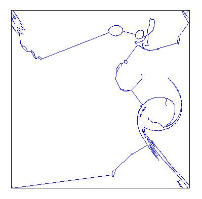
On a less formal note, these spanning tree constructions can be quite beautiful; minimal spanning trees of isosurfaces in sea surface vorticity, for instance, look remarkably like Miro drawings:
 |
 |
 |
In summary, these techniques provide an effective way to deduce connectedness properties of different objects from a finite amount of finite-precision samples of those objects. See the papers listed at the end of this page for more details.
One way to characterize the number and type of holes that a space contains is via its homology groups. The main ingredients in constructing the homology groups are a triangulation of the original space (called a simplicial complex) and a boundary operator that maps k-dimensional simplices onto the (k-1)-dimensional simplices in their boundary.
This figure illustrates the boundary operator acting on a 2-simplex to give a 1-chain, which is necessarily a 1-cycle:
A sum of k-simplices is called a k-chain. Any k-chain that has zero boundary is called a k-cycle. Some, but not all, k-cycles are the boundaries of (k+1)-chains. A k-dimensional hole is detected as a k-cycle that is not the boundary of a (k+1)-chain.
Not every non-bounding cycle represents a different "hole," so we need an equivalence relation that tells us which cycles go around the same hole. Indeed, two k-cycles are equivalent (or homologous) if their difference is the boundary of a k+1-chain. Algebraically, the k-th homology group is the quotient group of k-cycles by k-boundaries. The figure below shows a triangulation of an annulus. The inner blue 1-cycle is homologous to the outer perimeter, and each represent the homology class of the hole:
The k-th Betti number, b_k, is defined to be the rank of H_k, so it gives us the number of non-equivalent non-bounding k-dimensional cycles. b_0 is the number of connected components. For subsets of 3-dimensional space, b_1 is (roughly speaking) the number of open-ended tunnels, and b_2 is the number of enclosed voids. For the annulus example above, b_0 = 1, b_1 = 1, and b_k = 0 for all k>=2.
The first step is to fatten the data by forming its alpha-neighborhood (a union of balls of radius alpha centered at each data point), as shown above. This alpha-neighborhood is then partioned into cells by taking the intersection with the Voronoi diagram. The alpha shape is the geometric dual of the partitioned alpha neighborhood, where the duality operation is the same as that used to get the Delaunay triangulation from the Voronoi diagram. Thus, each alpha shape is a subset of the Delaunay triangulation.
A fast incremental algorithm due to Delfinado and Edelsbrunner computes Betti numbers of alpha shapes in R^2 and R^3. See Edelsbrunner's home page for more details.
Below on the left is an example alpha shape of 10^4 points on the
Sierpinski triangle. The blue outline is the border of the alpha
neighbourhood and the orange is the corresponding sub-complex of the
Delaunay triangulation. In the graphs on the right we plot the number
of connected components b_0(alpha) in blue and number of holes
b_1(alpha) in red.
The disconnected nature of the data is seen in the staircase growth of the blue curve (on the right) which counts the number of connected components. The graph of the number of holes (in red) shows that more holes are resolved as alpha decreases. What this graph fails to reveal however, is that the larger holes also disappear. The value of alpha for the neighborhood on the left is approximately 0.1. We can see three holes, and the graph of b_1 on the right records this. For alpha=0.2, the b_1 data shows there was a single hole. We can see that it would have been in the center of the fractal, but it is no longer present at the smaller alpha value chosen for the figure on the left.
This effect makes it difficult to make a correct diagnosis of the underlying topology. It does, however, give us geometric information about the embedding of the set in the plane, which may be useful in the context of some applications.
Mathematically, the problem is resolved by incorporating
information about how the fractal maps inside its alpha-neighbourhood,
or how a smaller neighbourhood maps inside a larger one. This leads
to the definition of a persistent Betti number, which was
introduced in V. Robins, "Towards computing homology from finite
approximations," Topology Proceedings 24 (and, somewhat
later, by Edelsbrunner and colleagues in
Disc. Comp. Geom. 28:511-533): for epsilon < alpha,
b_k(epsilon,alpha) is the number of holes in the epsilon-neighborhood
that do not get filled in by the alpha-neighborhood. Obviously, this is a
function of epsilon:
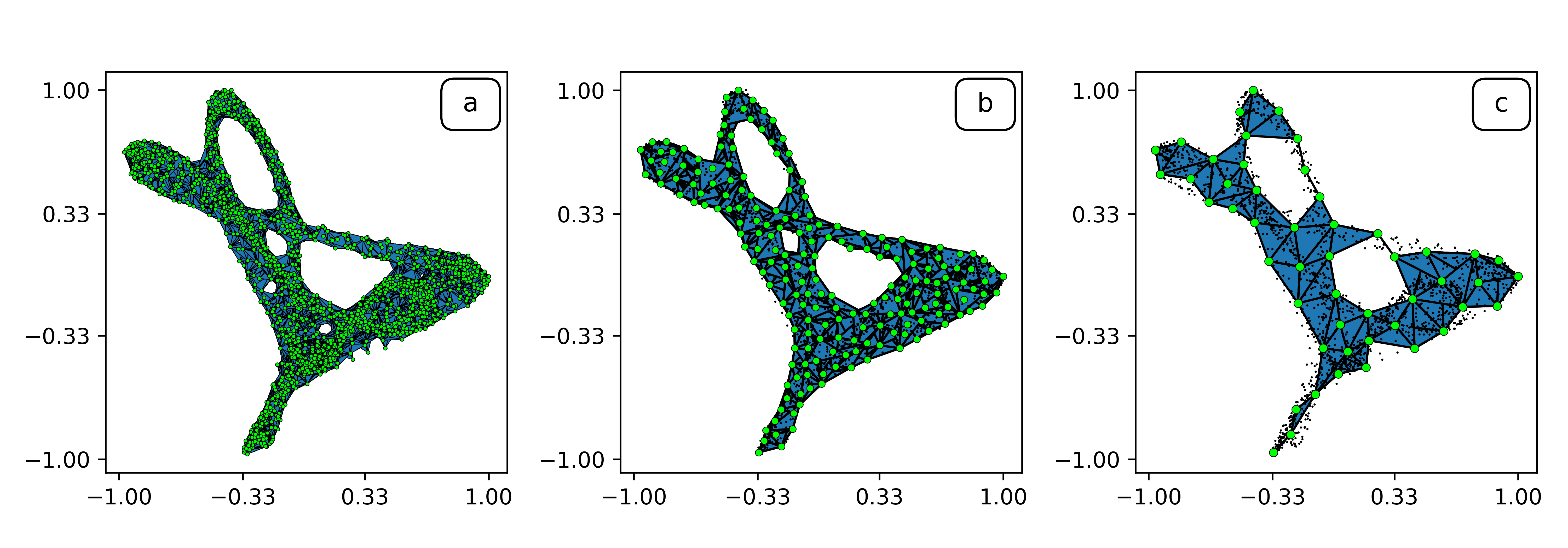
Images (b) and (c) above show witness complexes of the same trajectory, constructed using different values of epsilon.
Note that the alpha-neighborhood may have extra holes that were not present in the smaller neighborhood, but we are only interested in the holes that exist in both. For more details and a mathematically rigorous definition, see this paper or Vanessa's Ph.D. thesis (listed below).
The persistent Betti numbers are computable in principle using linear algebra techniques. Soon after the paper above came out, Edelsbrunner and collaborators made a similar definition of persistent Betti number for alpha shapes and devised an incremental algorithm for their quantity. See Edelsbrunner's home page for more details.
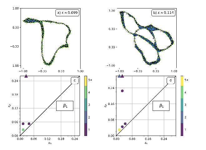
There are two useful representations that people use to capture
information about the formation and destruction of holes in a set as
the epsilon value is varied: the barcode and the persistence
diagram. The latter contains a single point for each hole; the x
coordinate is the epsilon at which the hole appears and the y
coordinate is the epsilon at which it disappears. The top row of the
image below shows witness complexes of trajectories from two dynamical
systems with associated persistence diagrams shown below.
Connectedness and noise are related in an interesting way, and so the techniques described above have some practical applications to filtering noise out of data. In particular, these variable-resolution connectedness studies address the scale of the separation between neighboring points, and noise is often "larger than" data. In that it brings out this kind of scale separation, the MST and the associated calculation of isolated points allows pruning of noisy points.
More formally, perfect sets by definition contain no isolated points, and most dynamical systems that are of practical interest have attractors that are perfect sets, so any isolated points in data from such systems are likely to be spurious.
This is particularly useful because simple low-pass filtering of data from chaotic systems - "bleaching" - is a very bad idea; check out this wonderful paper if that doesn't make sense to you.
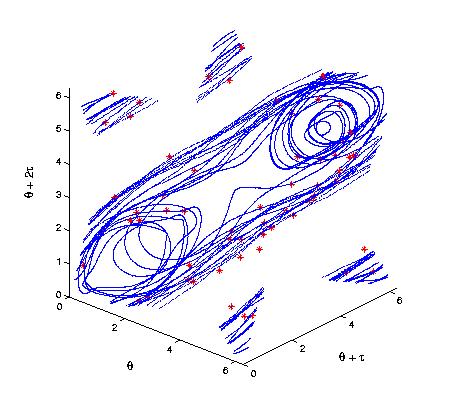
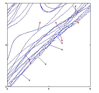
Below, to the left, is an experimentally measured trajectory of a chaotic pendulum. The bob angle was measured every several hundred milliseconds, and delay-coordinate embedding was used on this scalar data to reconstruct a diffeomorphic image of the attractor. The red points denote points that were altered by experimental error in the angle sensor. To the right is a close-up of the MST of this data set. Note how this construction makes the noisy points obvious: they are far from the rest of the trajectory, and in a transverse direction:
 |
 |
On the C(epsilon) and I(epsilon) graphs, this kind of noise manifests as an extra shoulder on the curves:
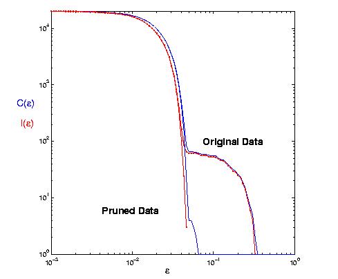 |
We have also applied our MST-based connectedness techniques to a number of other systems, including:
 |
In order to exploit this idea to pull a signal apart into its different regimes, one must come up with sensible approximations of "nearby" and "different" in the sentences above. Another challenge is that the components - clumps of "nearby" points - may overlap, causing their trajectories to locally coincide.
The 2011 CHAOS paper cited below demonstrates these ideas in the context of IFS, discrete-time dynamical systems in which each time step corresponds to the application of one of a finite collection of maps. In two examples - a Henon IFS and an experimental time series representing computer performance data - this segmentation algorithm accurately identifies the times at which the regime switches occur and determines the number and form of the deterministic components themselves. Finding holes in data sets has all sorts of interesting applications. The 2004 and 2017 Intelligent Data Analysis papers cited below, for exasmple, describe how these techniques can be used to characterize the distribution of melt ponds on the arctic ice sheet, to find leads and channels in the icepack, and to find safe paths through that icepack for a given size vessel and distinguish between the same note played on different musical instruments.
There are many other interesting applications of computational topology. Here are a few that we've thought about:
