CSCI 5854: Lecture 2 - Synchronous Models and Extended Finite State Machines

In this note, we will address the notion of synchronous models and present the model of extended finite state machines, which are a versatile model for synchronous systems.

Synchronous Systems

The term synchrony comes from the Greek words syn meaning "with" and kronos meaning time. As a result, synchronous models are models that are somehow synchronized to a clock. Synchronous models arise from digital computers.

A digital computer performs computation on a processor that has a clock which is a square wave oscillating at a fixed frequency. The computer performs its most fundamental (micro) operations such as reads/writes from register, ALU operations, reads from the bus when an edge (rising or falling edge) of the clock is encountered.

Synchronous systems abstract this concept further. We assume that time \(t\) is a non negative integer starting from \(t = 0\) and proceeding as \(t=1,2,3,\ldots\). Each time instant represents a clock edge, and all system operations happen at this very instant. We assume that the system's operations take no time whatsoever.

1. Example of a Synchronous Module

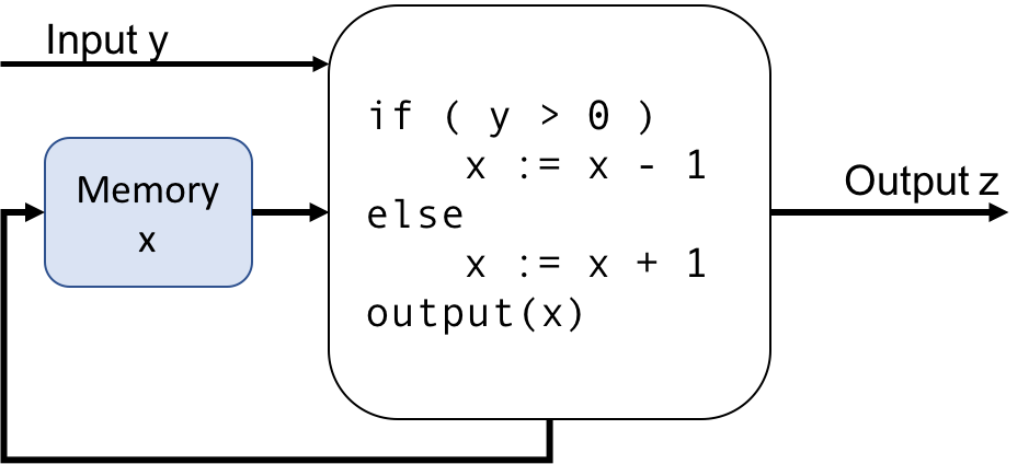
The figure below shows an example of a module with an input \(y\) internal state (memory) \(x\) and output \(z\). The module itself runs a C program at each time instant to calculate the new output \(z\) and the new value of the memory store.

Example of a synchronous module

Before the start, let us take \(x =1\). Suppose the inputs received are

At each time instant, the system the system receives a clock signal and processes its input. At \(t=0\), it receives \(y=1\). It calculates the new state \(x= 0\) and outputs \(z=0\). The system executes again at \(t=1, 2\) and so on. Overall, the value of \(x,z\) for the first \(8\) steps are as below.

Mathematical Definition

We will first define typed variables and their associated domains. A type such as int, real, bool refers to a set of values associated with the type. For instance, int refers to the set of integers, bool to the set \(\{T, F\}\).

Typed Variable

A typed variable \(x:\ \texttt{t}\) declares a variable \(x\) of type \(\texttt{t}\). For such a variable the set \(D(x)\) denotes the set of all possible values that \(x\) can take.

Example: Typed variable

The typed variable \(x: \texttt{int}\) declares a variable \(x\) such that \(D(x):\ \mathbb{Z}\), the set of all integers.

In our presentation, we will associate types to variables that are inputs, outputs and internal state variables for the synchronous systems we define. A typed variable \(x\) has a pre-defined type such as int, real, bool, string and so on. We associate \(x\) with a domain \(D(x)\) that refers to the set of possible values it can take. Likewise, given a set of variables \(X\), we use the shorthand \(D(X)\) to the product of the domains of each individual variables.

Synchronous Module

A (deterministic) synchronous module is defined by a tuple \((X, I, O, \delta, x_0)\), wherein

1. \(X\) is a set of typed internal state (memory) variables,
2. \(I\) is a set of typed input variables,
3. \(O\) is a set of typed output variables,
4. \(\delta: D(X) \times D(I) \rightarrow D(X) \times D(O)\) is a function such that \(f(x,i) = (x',o)\) maps current state \(x\) and input \(i\) to next state value \(x'\) and output \(o\), and
5. \(x_0 \in D(X)\) represents the initial state of the system.

Going back to the example (1) above, we have

1. \(X\ =\ \{x:\ \texttt{int}\ \}\)
2. \(I\ =\ \{y:\ \texttt{int}\ \}\)
3. \(O\ =\ \{z:\ \texttt{int}\ \}\)
4. \(\delta\) is defined by the execution of the program shown in the example.

\[\delta(x,y):\ \begin{cases} (x-1, x-1) & \text{if}\ y > 0\\ (x+1, x+1) & \text{if}\ y \leq 0 \\ \end{cases} \]

5. \(x_0\) is the state \(x: -1\).

Executions of a deterministic synchronous module

An execution of a deterministic synchronous module \((X, I, O, \delta, x_0)\) given a sequence of inputs \[ i(0), i(1), i(2), i(3), \ldots \]

is a sequence of pairs \(( x(j), o(j) )\) for \(j=0,1,\ldots,\) such that

1. \((x(0), o(0)) = \delta(x_0, i(0))\) for the initial time \(t = 0\)
2. \((x(t+1), o(t+1)) = \delta(x(t), i(t))\) for all times \(t \geq 0\).

In other words, the systems state before the time \(t = 0\) is \(x_0\). The subsequent states starting from \(x(0), \ldots\) and the subsequent outputs \(o(0), o(1), \ldots\) are all obtained by applying the transition relation on the previous state of the system.

However, the mathematical definition provided above is quite general, and will cover every synchronous model imaginable. However, it is also quite unwieldy. Simply put, it is good for simple example but does not help us model more complex examples. Therefore, we will use the visual model of extended finite state machines to model synchronous systems.

Extended Finite State Machines (EFSMs)

EFSMs are a simple and natural class of models for synchronous systems. An EFSM models a synchronous system using a state machine which has finitely many modes (also known as states) and transitions (edges) between them.

@(ex4) Example of an EFSM

Consider the system shown below.

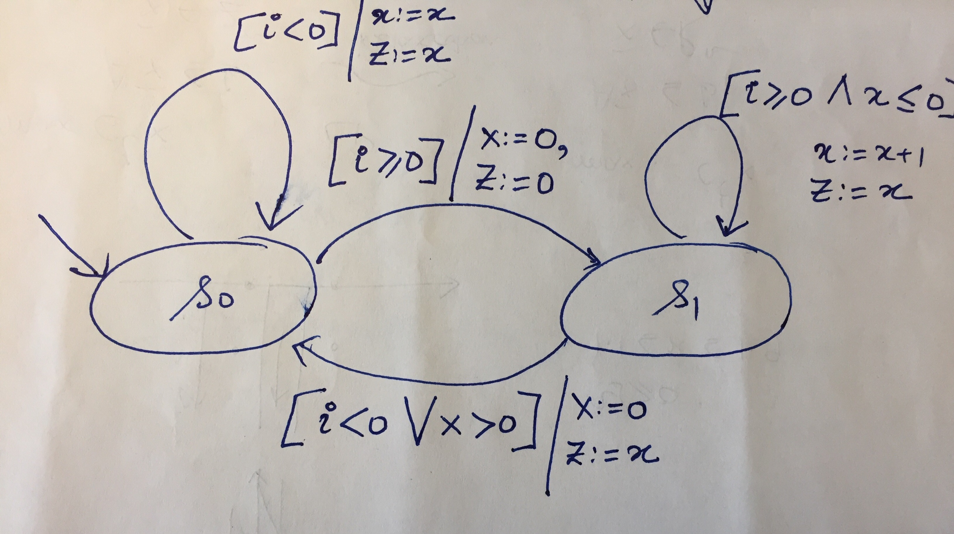
Extended Finite State Machine Example

The system defines a synchronous module.

1. It has input variable \(i: \texttt{int}\)
2. Output variable \(z: \texttt{int}\).
3. The internal state variable is \(x: \texttt{int}\).
4. Another internal state variable of all EFSMs is the \(\texttt{mode}\) of the system \(\texttt{mode}: \{ s_0, s_1\}\) which can either be \(s_0\) or \(s_1\).
5. The initial state of the system is \((\texttt{mode}: s_0, x : 0)\).
6. The transition function of the system is defined by the arrows in the diagram.

Let us look in isolation at one of the arrows below.

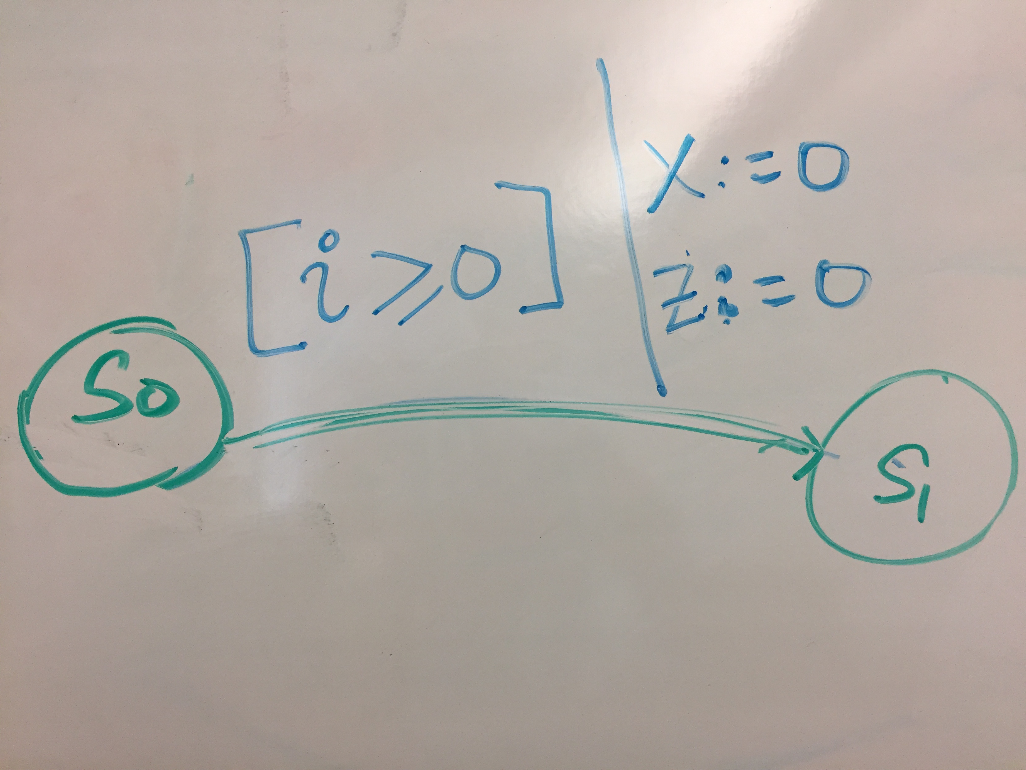
Transition Edge in an EFSM

The arrow goes from \(s_0\) to \(s_1\). The part \([i \geq 0]\) is the guard of the transition and the assignments \(x := 0, z := 0\) represent the updates made by the transition.

Transition Syntax

Each transition has the following syntax

[guard condition]/{action}

The guard condition can involve a Boolean predicate over the input and internal state variables of the EFSM, and specifies what needs to be true about the input and the internal state for the transition to be enabled. The action specifies assignment to the output and internal state variables when the transition is taken.

Extended Finite State Machine (EFSM)

An Deterministic EFSM is a tuple \((Q, X, I, O, s_0, x_0, \delta)\) with the following components

1. \(Q: \{ s_1, \ldots, s_m \}\) is a finite set of modes (sometimes confusingly called states).
2. \(X: \{ x_1: {\tau_1}, \ldots, x_n: {\tau_n}\}\) represents the typed internal state variables.
3. \(I: \{ i_1: {\tau_1}, \ldots, i_k: {\tau_k}\}\) represents the input variables.
4. \(O: \{ z_1: {\tau_1}, \ldots, z_l: {\tau_l}\}\) represents the typed output variables.
5. \(s_0 \in Q\) is the starting mode; and \(x_0 \in D(X)\) is the initial value of the internal state variables.
6. \(\delta: Q \times D(X) \times D(I) \rightarrow Q \times D(X) \times D(O)\) is the transition function wherein \(\delta(q, x, i) : (q', x', z)\) denotes that from the mode \(q\), internal state value \(x\), input value \(i\), we move in a step to \(q' \in Q\), \(x' \in D(X)\) and output the value \(z \in D(O)\).

Going back to Example @(ex4), we have

• \(Q = \{ s_0, s_1\}\),
• \(X = \{ x: \texttt{int} \}\),
• \(I: \{ i: \texttt{int}\}\),
• \(O: \{ z: \texttt{int}\}\),
• \(q_0: s_0\),
• \(x_0: 0\) and
• The transition function \(\delta\) as below:

\[ \delta(i, q, x): \left\{\begin{array}{cccl|l} q' & x' & z \\ (s_0, & x, & x ) & \text{if}\ q = s_0\ \land\ i < 0 & \texttt{self loop on }\ s_0\\ (s_1, & 0, & 0 ) & \text{if}\ q = s_0\ \land\ i \geq 0 & \texttt{edge from}\ s_0 \rightarrow s_1\\ (s_1, & x+1,& x) & \text{if}\ q = s_1\ \land\ i \geq 0\ \land x \leq 0 & \texttt{self loop on}\ s_1\\ (s_0, & 0, & x ) & \text{if}\ q = s_1\ \land\ (i < 0\ \lor\ x > 0) & \texttt{edge from}\ s_1 \rightarrow s_0\\ \end{array}\right.\]

Deterministic EFSM

An EFSM is deterministic if and only if the following conditions hold:

1. It has a single initial mode \(s_0 \in Q\),
2. It has a single initial internal state \(x_0 \in D(X)\),
3. For every mode \(s\), consider the guard conditions \(\varphi_1, \ldots, \varphi_j\) on its outgoing transitions (edges)

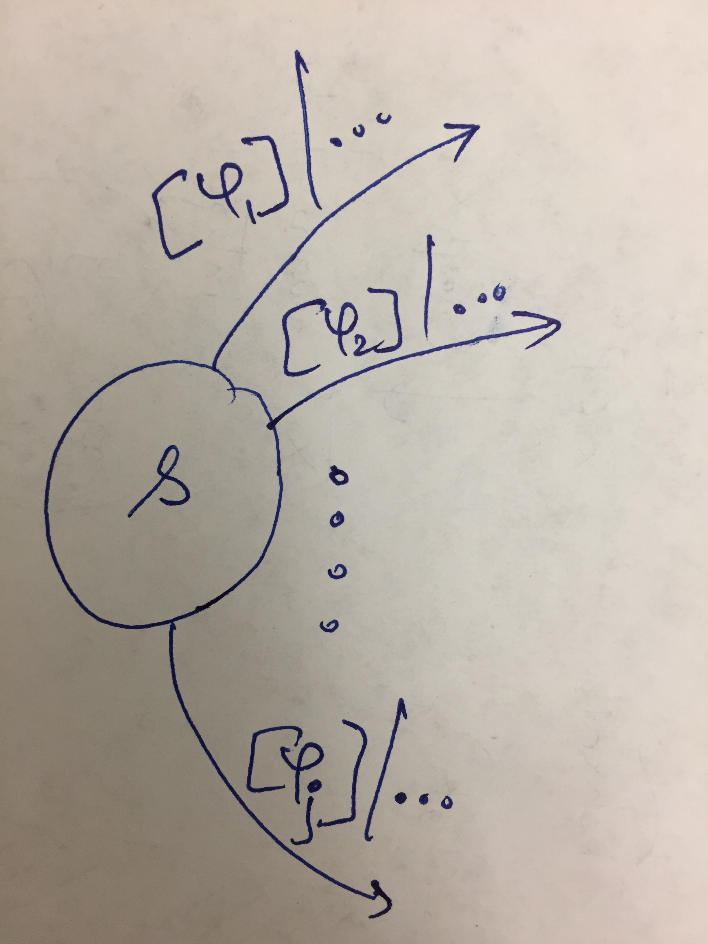
Outgoing transitions from state \(s\)

The guard conditions satisfy the following.

• The guard conditions satisfy mutual exclusion: \(\varphi_i\ \land\ \varphi_j\ \equiv \ \text{false}\).
• The guard conditions are mutually exhaustive: \(\varphi_1 \ \lor\ \cdots \ \lor \varphi_j\ \equiv\ \text{true}\).

Check that these conditions are actually true for the example of EFSM above. In particular, the guards on the ougoing edges of \(s_1\) are

• $_1: i 0   x 0 $.
• \(\varphi_2:\ i < 0\ \land\ x > 0\).

Verify that \(\varphi_1 \land \varphi_2: \text{false}\) and \(\varphi_1 \lor \varphi_2: \text{true}\).

Concluding Remarks

Thus far, we have defined a deterministic synchronous module and the model of deterministic extended finite state machines. In the subsequent section, we will look into nondeterministic models, introduce event types and talk about compositions of these systems.